This article details how to use Simcenter Testlab Signature (formerly called LMS Test.Lab) to measure data on a piece of rotating machinery. Possible measurement functions include orders and spectral waterfall functions. These functions show the evolution of vibration or sound as a function of speed of the rotating object.
A minimum of two channels of data are required to measure spectral waterfalls and orders:
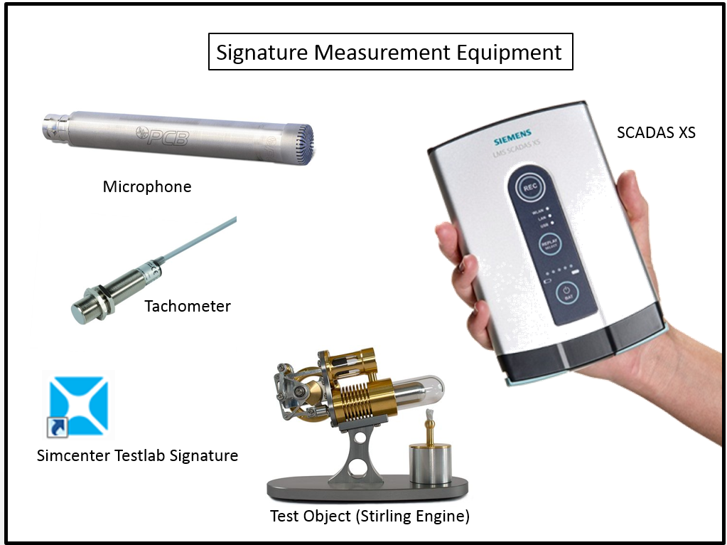
The speed of a rotating piece of machinery is measured in revolutions per minute, or RPM, by the tachometer. The sound and/or vibration of the rotating system is measured in conjunction with the tachometer, using microphones and accelerometers.
Equipment Needed
Here is a complete list of required equipment (Figure 1):

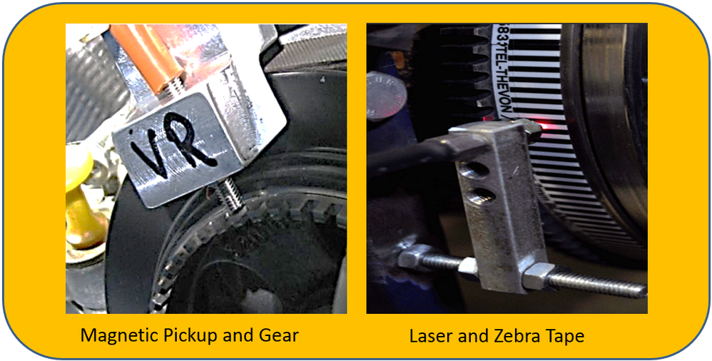
Depending on the test object, different types of tachometers might be used (Figure 2). For example, magnetic pickups are ideal for metal gears, while lasers are often used with striped “zebra tape”.
A tachometer measures speed in revolutions per minute or RPM. The tachometer sensor detects when a gear tooth, piece of reflective tape, or stripe passes by the sensor as shown in Figure 3.
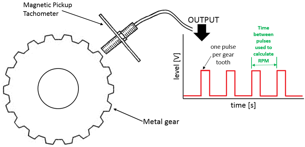
Using the time between crossings, the Simcenter Testlab software can calculate the speed at which the shaft is rotating in units of RPM.
Getting Started
The following channels should be in place:
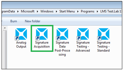
To get started with Simcenter Testlab Signature:
Note: It is also possible to copy this icon onto your desktop to create a shortcut. Right click on the icon and select “Send to -> Desktop (create a shortcut)”.
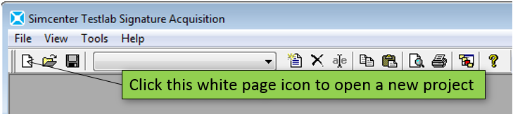
Once the software is open, a mostly grey screen appears, waiting for a project to be opened. Click the white page icon in the top left to open a new project as shown as in Figure 5. The software will communicate to the SCADAS frontend to determine the number of available channels for the test. This can take a few seconds depending on the number of channels.
After the new project is open, it is called “Project1.lms” by default. This is similar to how Microsoft Powerpoint starts with “Presentation1.pptx” or Microsoft Word starts with “Document1.docx”. Choose “File -> Save As…” from the main menu to save a project to the desired name as shown in Figure 6. The project file will have an *.lms extension and can be stored in any directory.
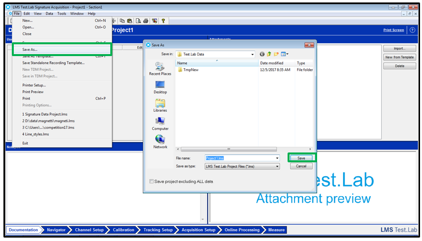
There are several ‘worksheets’ along the bottom of the screen as shown in Figure 6. To setup and perform a signature measurement, work through the worksheets from left to right, starting with the ‘Documentation’ worksheet and ending in the ‘Measure’ worksheet. Note that the Navigator worksheet, which is used for data viewing, can be skipped until some data is acquired.
In the ‘Documentation’ worksheet, pictures of the test setup can be stored and other documentation created. See the Knowledge Base article called “What’s up with the Documentation worksheet?”.
Channel Setup
After documenting, select the ‘Channel Setup’ worksheet as shown in Figure 7. An Excel-like table contains a list of all the channels in the connected SCADAS frontend. Each row corresponds to one channel.
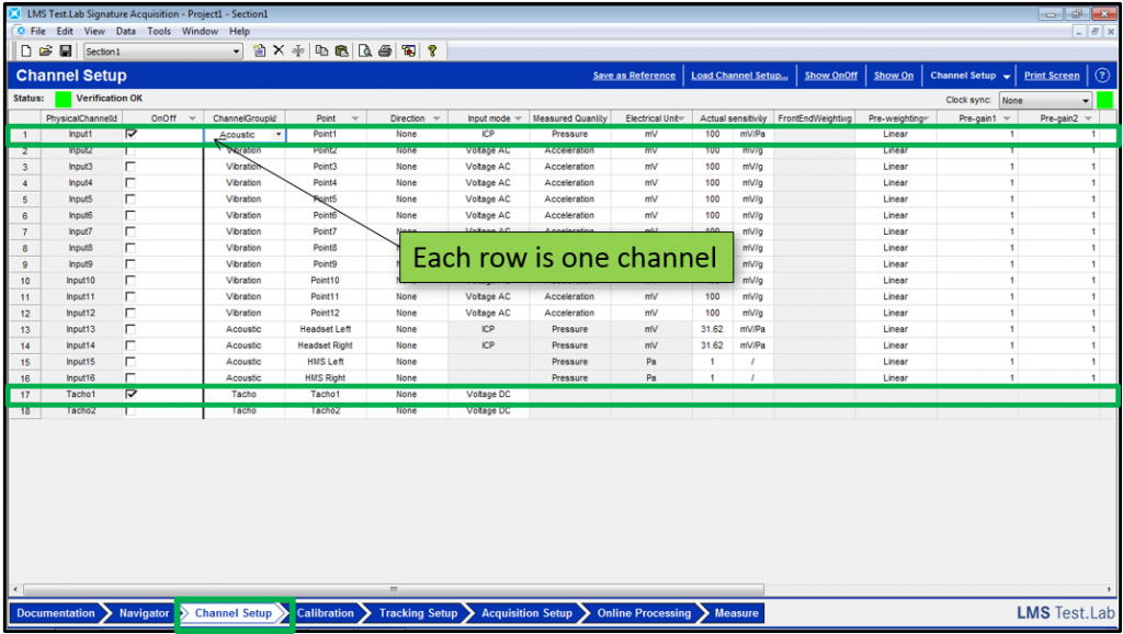
Turn ON the Input1 and Tacho1 channels by checking the box next to each input name:
If triaxial accelerometers are being used, see the Knowledge Base article: “Cool triaxial accelerometer tips” for some useful setup tips.
Now the microphone can be calibrated before taking the measurement.
Calibration
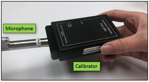
A pistonphone can be used to calibrate the microphone. The pistonphone produces a specific frequency and amplitude level to check the calibration of the microphone and adjust it if necessary.
At the top of the ‘Calibration’ worksheet, enter the specific information for the calibrator being used (Figure 8).
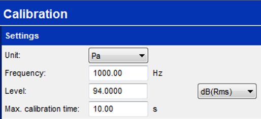
The unit for a microphone calibrator is “Pa” which is an abbreviation for the sound pressure measurement unit of Pascals. In this case, 1000 Hz and 94 dB RMS are settings from the calibrator. The frequency of 1000 Hz is common for microphone calibrators because the A-weighting curve has 0 dB of attenuation or gain at that frequency, so it cannot affect the calibration value.
Insert the microphone into the calibrator as shown in Figure 9.
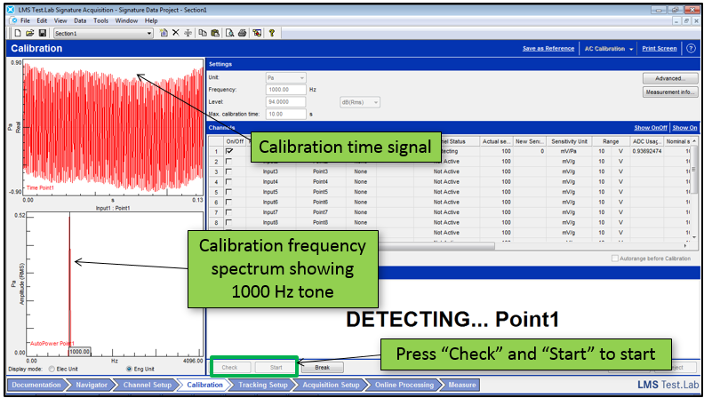
After entering the calibrator values, turn on the calibrator, and press the “Check” and “Start” buttons at the bottom of the worksheet as shown in Figure 10. The calibration time history and frequency spectrum should show on the left hand side.
If the calibrator frequency measures as expected, the calibration starts. An orange message will indicate that calibration is in progress as shown in Figure 11.
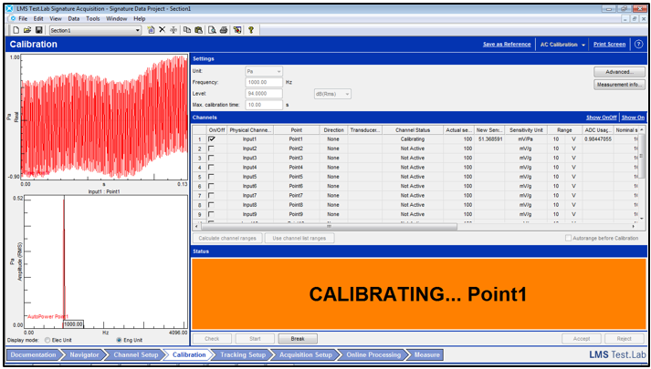
This orange message area is designed to allow viewing from across a room so a single person can do the calibration.
When the calibration is finished, the message area turns green as shown in Figure 12.
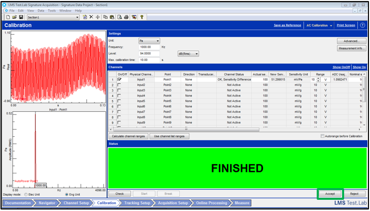
The newly calculated calibration values are shown in a column called “New Sensitivity”.
The previous calibration values are shown in the column labelled “Actual Sensitivity”. The “Actual Sensitivity” values are used for the measurement.
Press the “Accept” button (lower right) to update the calibration values. The values in “New Sensitivity” will replace the values in “Actual Sensitivity”. These values will automatically be active everywhere in Simcenter Testlab, including the ‘Channel Setup’ worksheet.
The left side displays will also update to reflect the new calibration values.
Tracking Setup
In the ‘Tracking Setup’ worksheet, there are two main objectives:
Tachometer Setup
Set the pulses per revolution on the right hand side to match the number of pulses per revolution of the tachometer being used. In this example, the number of pulses is set to 1. The tachometer calculates RPM using only the one piece of tape placed on the flywheel of the stirling engine.
With the test object running, set the trigger level for the tachometer as shown in Figure 13. The black line, which is a graphical representation of the trigger level, should ideally be placed in the center of the pulses.
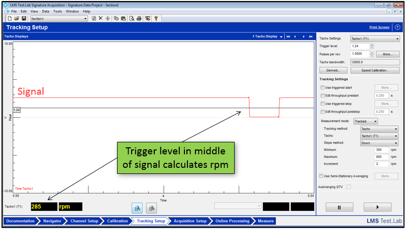
If the trigger is set properly, the yellow RPM readout in the lower left should read close to the expected RPM value.
The trigger level can be changed if the RPM is not reading properly. The trigger level can be lowered or raised by:
If the trigger is set too high or too low, the tachometer will read zero RPM as shown in Figure 14.
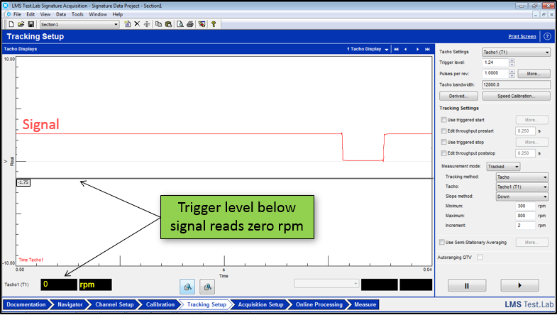
Set the trigger level to where the tachometer pulse passes through the signal and the RPM reads out properly at the bottom of the tracking screen.
Tracking Setup
The type of results, as well as the start and stop conditions of the measurement, are set in the Tracking setup area in the lower right of the worksheet. Examples of possible start and stop conditions include:
In addition to start and stop definition, there are two options for measurement output that can be defined: tracked and stationary (Figure 15):
If both a tracked result and stationary result are desired, this is possible. The measurement mode should be set to tracked, and ‘Map statistic’ functions should be checked on. The ‘Map Statistic’ function can be enabled in the Online Processing worksheet in the Sections area under Map Statistics.

In this example, measurement mode will be set to tracked to measure a run down from 800 RPM to 300 RPM, with the increment setting of 2 RPM. The data will be collected from 800 rpm to 300 rpm with a spacing of 2 RPM between each spectrum in the resulting waterfall. Approximately 250 spectrums will be calculated during the measurement (500 RPM range divided by increment of 2). In reality, the 2 RPM is a decrement, not an increment, in this example.
Acquisition Setup
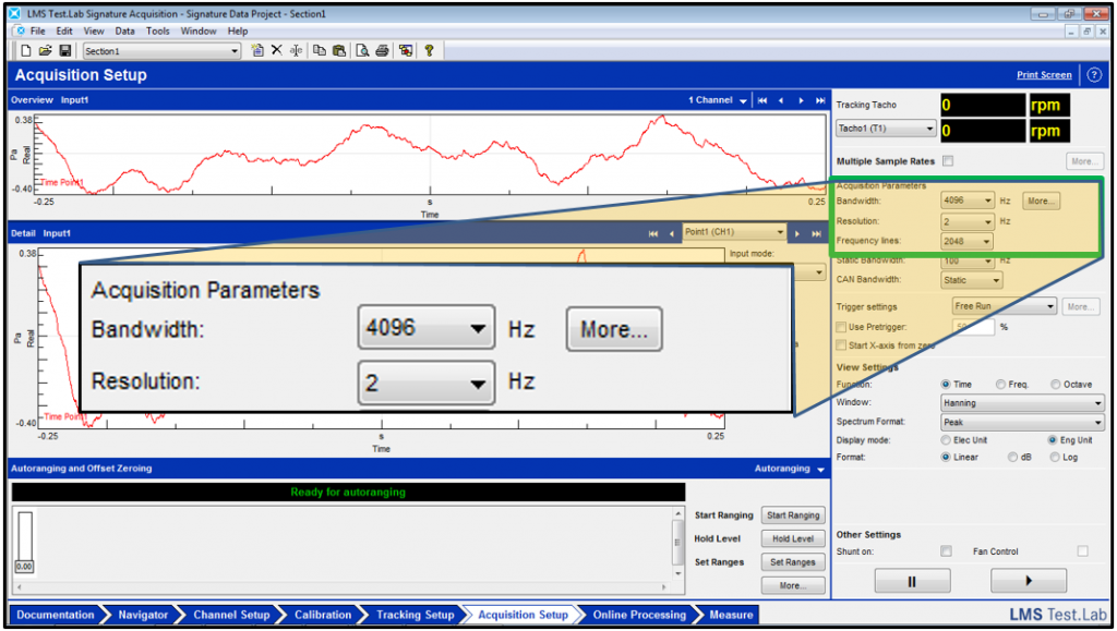
Move to the ‘Acquisition Setup’ worksheet as shown in Figure 16. Here the bandwidth and frequency resolution for the Fourier spectrums can be set:
***Important: Set the sampling rate high enough to capture any frequency of interest, because it is difficult to re-measure later once the test object is de-instrumented and sent away.***
If the measurement consists of both acoustic and vibration signals, different sampling rates can be set for each type of signal. Check on the ‘Multiple Sample Rates’ checkbox in the upper right corner of the software.
See the ‘Digital Signal Processing’ Knowledge Base article for more information on sampling rates, frequency resolution, bandwidth, etc.
Online Processing
Move to the ‘Online Processing’ worksheet. It is possible to have the Simcenter Testlab Signature software process the data while it is being acquired. For example, go to the acoustic tab at the top of the worksheet and change the ‘Final weighting’ to A-weighting as shown in Figure 17.
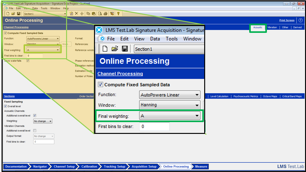
By setting A-weighting in the Acoustic group, any spectrums calculated from the acoustic channels will be A-weighted, even if the time data is being acquired with Linear weighting.
Some additional notes about weighting with Simcenter Testlab:
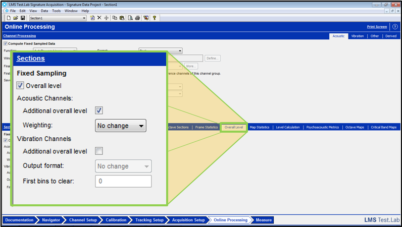
Additional processing functions, like overall level and orders, can be calculated while the acquisition is on-going. Go to the ‘Overall Level’ tab in the middle of the worksheet and make sure the ‘Overall Level’ checkbox is checked ON as shown in Figure 18.
In the ‘Order Sections’ tab, enter the orders to be calculated. For example, entering “1;2;3;4;5;6” will create a table of six orders to be calculated. Make sure to press ENTER or the orders will not be calculated.
If the orders have been entered correctly, a table should appear as shown in Figure 19.
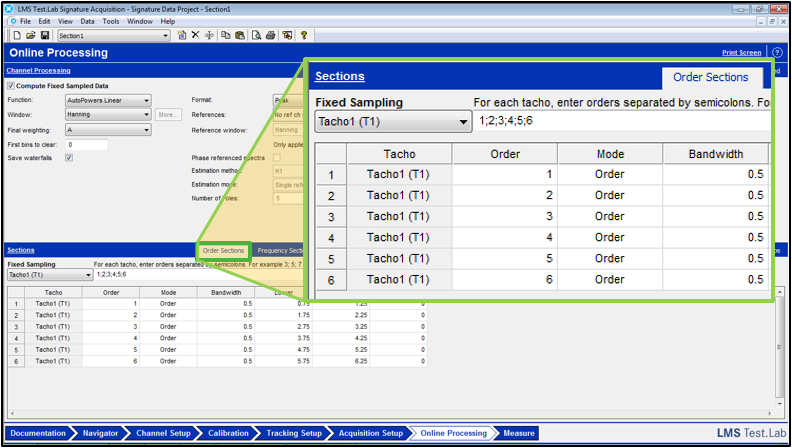
After pressing enter, the table should be filled in with the orders. The cut mode for the orders and corresponding bandwidth can be entered. If there is more than one tracking tachometer, it can be selected in the upper left of the menu. Orders with respect to each separate tachometer can be entered.
There are many other calculations that can be done while the measurement is in progress, including psycho-acoustic metrics, frequency band cuts, frame statistics, and derived channels.
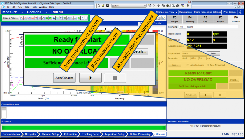
Measure
In the Measure worksheet, the acquisition is performed. All settings from previous worksheets are used in this worksheet. There are some Function buttons across the top where these settings can be changed (F3, F4, F5, F6, F8). Any changes performed with the function buttons are cascaded automatically to all related worksheets.
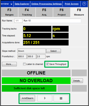
In the lower right, there are buttons to start and stop the acquisition as shown in Figure 20. Displays can be setup to monitor the data while acquiring.
Throughput
Make sure that the check box that says ‘Save Throughput’ is checked as shown in Figure 20. Checking this ON saves raw throughput time data for listening and re-processing at a later time.
In addition to collecting the throughput time file, the processed data will also be calculated during the measurement. Be sure that under “Tools -> Add-ins” that the “Time Recording during Signature” add-in is turned ON, otherwise an error message may appear, especially if this is the first time the software is being used.
Displaying Data while Measuring
Displays can be configured to monitor and view data while measuring (Figure 21). To do so:
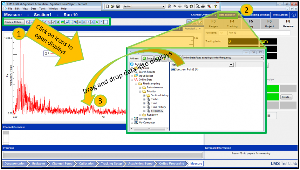
There are several folders in the ‘Online Data’ folder:
For more information on creating and changing display layouts, see the “Simcenter Testlab Display Layouts” Knowledge Base article.
Acquiring Data
To begin the measurement, use the buttons on the middle of the right hand side. Press the ARM button and then the PLAY (with arrow) button (Figure 22). This will start the measurement. When the start trigger condition is reached, the displays should update.
When the rundown has finished, press “Yes” to accept the data and then press ARM button again to disarm.
Post Processing Data: Processing Cursor
Use the processing cursor to interrogate the data (Figure 23):
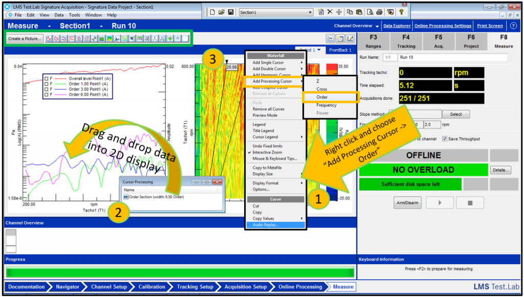
More information on the Processing cursor can be found in the Knowledge Base article ‘Interactive Order Cursor!’.
Post Processing Data: Audio Replay
It is possible to listen to the recorded data and filter it while listening (Figure 24):
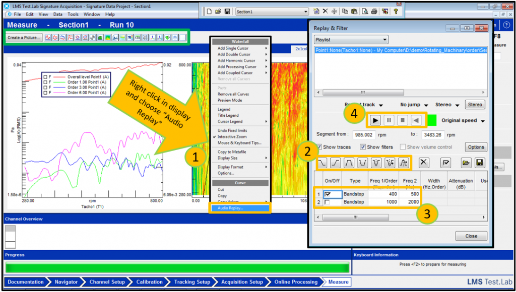
When listening, filters can be turned ON and OFF using the checkbox next to the filter type.
If Audio Replay does not appear when right clicking, make sure to turn it on under “Tools -> Add-ins”. Select “Audio Replay and Filtering”.
If performing multiple runs and statistics, the “Run Data Averaging and Comparison” organizer under “Tools -> Add-ins” is very helpful. It can be used to capture the maximum, average, minimum, and six sigma standard deviation of the runs. More information is available in the ‘Compare runs’ Knowledge Base article.
Questions? email us on hotline@dagtech.com.my, or contact Siemens Support Center.